Caffeine optimization

The question

If you drink coffee every week, which schedule gives the most productivity over a month? More caffeine helps now. It also builds tolerance and damages sleep, and both of them cost productivity later.

This was my IB Extended Essay. I wrote the model as a differentiable program and let gradient descent find the schedule.

The model

The variables are a weekly schedule of doses. There is one dose slot every 4 hours, so a week has 42 slots. The model repeats the week for 28 days and simulates it in steps of 5 minutes. Thus a schedule that works for one day but builds tolerance over a month gets a low score.

Concentration. One dose gives a blood concentration that rises and then decays:

$$C(t) = A\left(e^{-k t} - e^{-k_a t}\right), \quad A = 3.6472,\; k = 0.001393,\; k_a = 0.0603$$

Doses are relative to 160 mg. The concentrations of all doses add up. A weight matrix $W$ holds the contribution of each weekly slot to each 5-minute step of the month. I calculate it once. Each training step is then one matrix-vector product:

$$\vec{C} = W \, \frac{\vec{V}}{160}, \qquad W_{j,i} = C\big((j\,d_m - i\,d_w) \bmod W_m\big)$$

Tolerance. Tolerance follows the concentration with a first-order equation. I step it forward with the Euler method and clamp it to $[0, 1]$:

$$T_{i+1} = T_i + d_m\, k_t \left(C_i - T_i\, C_{tol}\right)$$

Effect. The effect saturates at high concentration, and tolerance reduces it:

$$E(t) = E_{max}\,\frac{C(t)}{EC_{50} + C(t)}\,\big(1 - T(t)\big)$$

Base productivity. A daily sine wave, lower in the morning and higher in the evening:

$$P(t) = 0.5 \sin\!\left(\frac{2\pi}{1440}\big((t \bmod 1440) - 960\big)\right) + 1$$

Sleep deprivation. A second state changes only during sleep hours. If the caffeine effect during sleep is above a threshold, the deprivation increases. If it is below the threshold, the deprivation decreases back to the rested value of 1. A sigmoid makes this step differentiable.

Reward. Productivity, divided by the sleep deprivation, times the caffeine effect:

$$R = \sum_t \frac{P_t}{SD_t}\,\big(1 + E_t\big)$$

Optimization

The 42 doses are an nn.Parameter in PyTorch. The loss is $-R$. Adam changes the doses for 600 epochs, and the doses are clamped at zero.

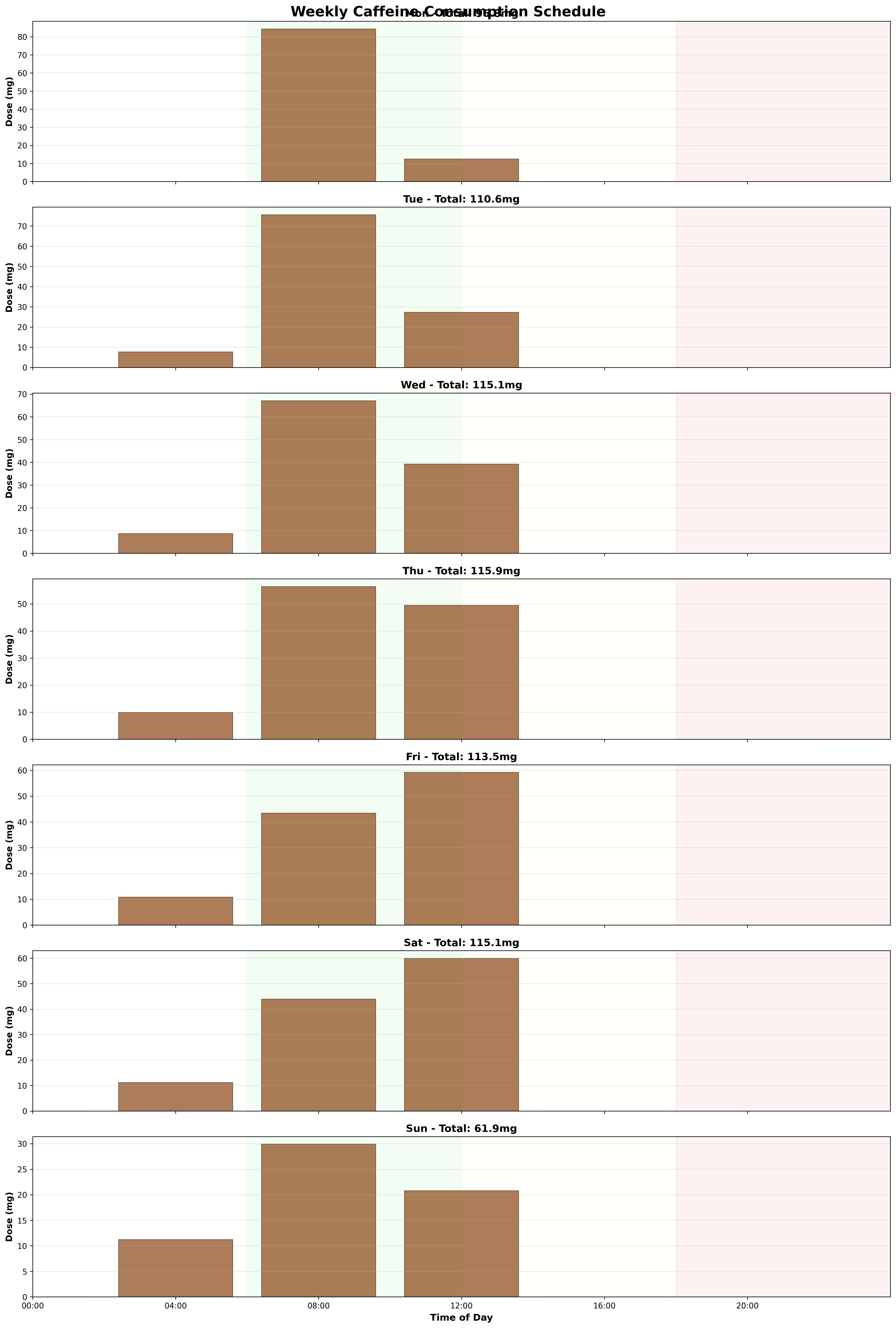
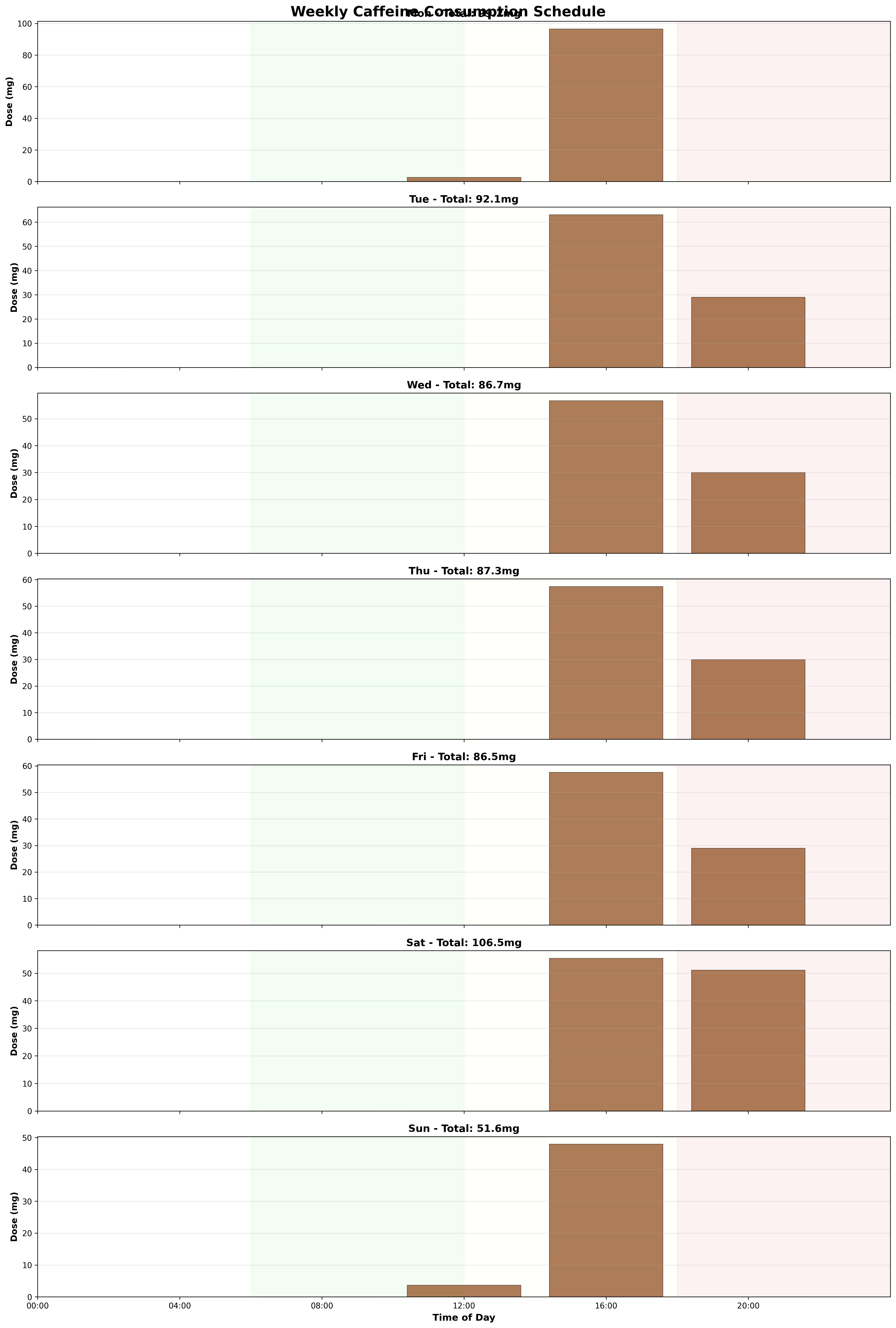
A single dose can reduce productivity much later, through the sleep state. Gradient descent finds these effects without special rules.

The study

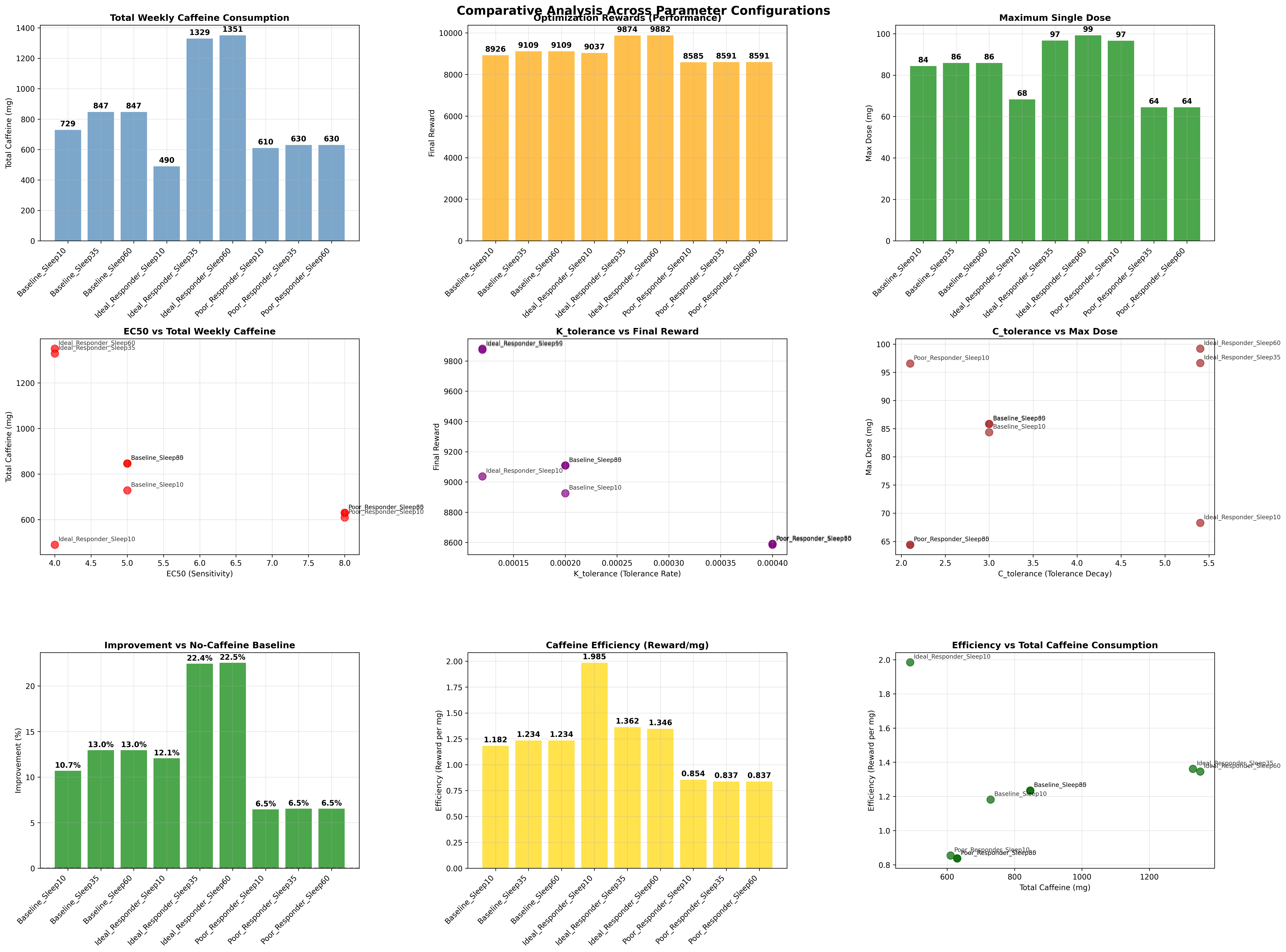
I ran 9 configurations. There are 3 responder profiles ($EC_{50}$ = 4, 5 and 8, with their own tolerance parameters) and 3 sleep thresholds (0.10, 0.35 and 0.60). Each run also has a baseline without caffeine for comparison.

Limits

The result depends on the parameters. The 9 configurations show how much the best schedule changes when the parameters change. The result is a method, not medical advice.