Caffeine Optimization

This project models repeated caffeine dosing as a constrained optimization problem. The objective is to choose a weekly dosage schedule that maximizes modeled productivity over a longer repeated horizon while accounting for:

• blood caffeine concentration,
• diminishing effect due to tolerance,
• baseline circadian productivity,
• sleep-deprivation penalties,
• dose timing and magnitude.

I'll work on reorganizing the files and uploading into GitHub in the future because right now it's too messed up.

Model overview

The model is a sequence of dependent subsystems:

1. A vector of editable dose variables defines a weekly schedule.
2. A concentration model maps each dose into a blood-concentration contribution over time.
3. Contributions from all doses are superposed into a full concentration time series.
4. A tolerance state is advanced sequentially from the concentration series.
5. A saturating caffeine-effect function combines concentration and tolerance.
6. Baseline productivity is defined as a circadian sinusoid.
7. Sleep deprivation evolves through a separate time-dependent recurrence.
8. The final reward combines effective productivity and caffeine effect over the optimization horizon.

Concentration model

The model assumes that the concentration contribution from one dose can be approximated by a biexponential rise-and-decay function:

C(t) = A * (exp(-k * t) - exp(-k_a * t))

The selected parameters in the manuscript are:

A = 3.6472
k = 0.001393
k_a = 0.0603

The code normalizes dose magnitudes relative to a 160 mg base dose, then superposes shifted concentration responses across time.

Weekly dose variables and month-scale evaluation

The optimized parameter vector is a weekly schedule:

V = [V_0, V_1, ..., V_n]

Each element represents the caffeine dose at one weekly decision slot. The final implementation uses a 4-hour spacing between available weekly dose slots, which avoids unrealistic schedules with arbitrarily precise minute-level dosing.

However, the reward is not evaluated over only one week. The weekly schedule is tiled across a 28-day window. This forces the optimizer to account for accumulated tolerance and repeated sleep effects rather than maximizing an isolated short-term day.

Weight-matrix construction

The concentration series is computed through a fixed weight matrix:

C_vector = W * (V / 160)

Each matrix entry represents the concentration contribution at one monthly time step from one weekly dose slot:

W[j, i] = C((j * d_m - i * d_w) mod W_m)

Where:

• $d_m$ is the monthly simulation time step,
• $d_w$ is the weekly dose spacing,
• $W_m$ is the number of minutes in a week.

The important computational point is that W is precomputed once. Training iterations then reuse a matrix-vector multiplication rather than recomputing all concentration contributions individually. The implementation uses:

• 5-minute simulation resolution for the 28-day dynamics,
• 4-hour dose-slot resolution for the optimized weekly schedule.

Tolerance dynamics

Tolerance is modeled with a first-order update:

dT/dt = k_t * (C(t) - T * C_tol)

After discretization with forward Euler:

T[i + 1] = T[i] + d_m * k_t * (C[i] - T[i] * C_tol)

In code, the tolerance vector is computed sequentially because each state depends on the previous tolerance value. The result is clamped into the range $[0,1]$.

Caffeine-effect function

Effect is calculated with a saturating dose-response term and a tolerance multiplier:

E(t) = E_max * (C(t) / (EC_50 + C(t))) * (1 - T(t))

The concentration term expresses diminishing returns at higher concentration. The tolerance term reduces the achieved effect as the model accumulates repeated exposure.

Productivity baseline

Baseline productivity is represented by a sinusoid:

P(t) = A * sin((2 * pi / P) * ((t mod P) - phi)) + V

The chosen parameters in the manuscript are:

• amplitude $A=0.5$,
• period $P=1440$ minutes,
• phase shift phi = 960 minutes,
• vertical shift $V=1$.

This creates a strictly positive baseline productivity curve with lower values in the morning and higher values in the evening.

Sleep-deprivation state

There's a sleep-deprivation state updated only during sleep hours using a sleep mask and a differentiable sigmoid-based relation between caffeine effect and sleep quality. A state recurrence advances the deprivation value over the monthly window, clamps the result to remain at or above the rested baseline, and divides productivity by the resulting factor.

In simplified terms:

• higher effect during sleep-associated intervals increases the sleep penalty,
• lower effect allows the sleep-related term to move the system back toward baseline,
• the reward function then receives a productivity signal already degraded by accumulated sleep state.

The exact implementation is not a simple static penalty. It is a time-evolving state sequence, which means one dose can affect downstream productivity indirectly through the sleep-deprivation path.

Reward function and optimization

The final reward combines productivity and caffeine effect:

R = sum_t ((P[t] / SD[t]) * (1 + E[t]))

The optimizer maximizes this reward by minimizing the negative reward:

loss = -R

The PyTorch implementation places the weekly caffeine-dose vector in an nn.Parameter, computes the differentiable forward model, performs backpropagation, and updates doses using Adam.

The optimization loop logs dose statistics over training, stores the final latent trajectories, and exports schedule data and comparison outputs for later analysis.

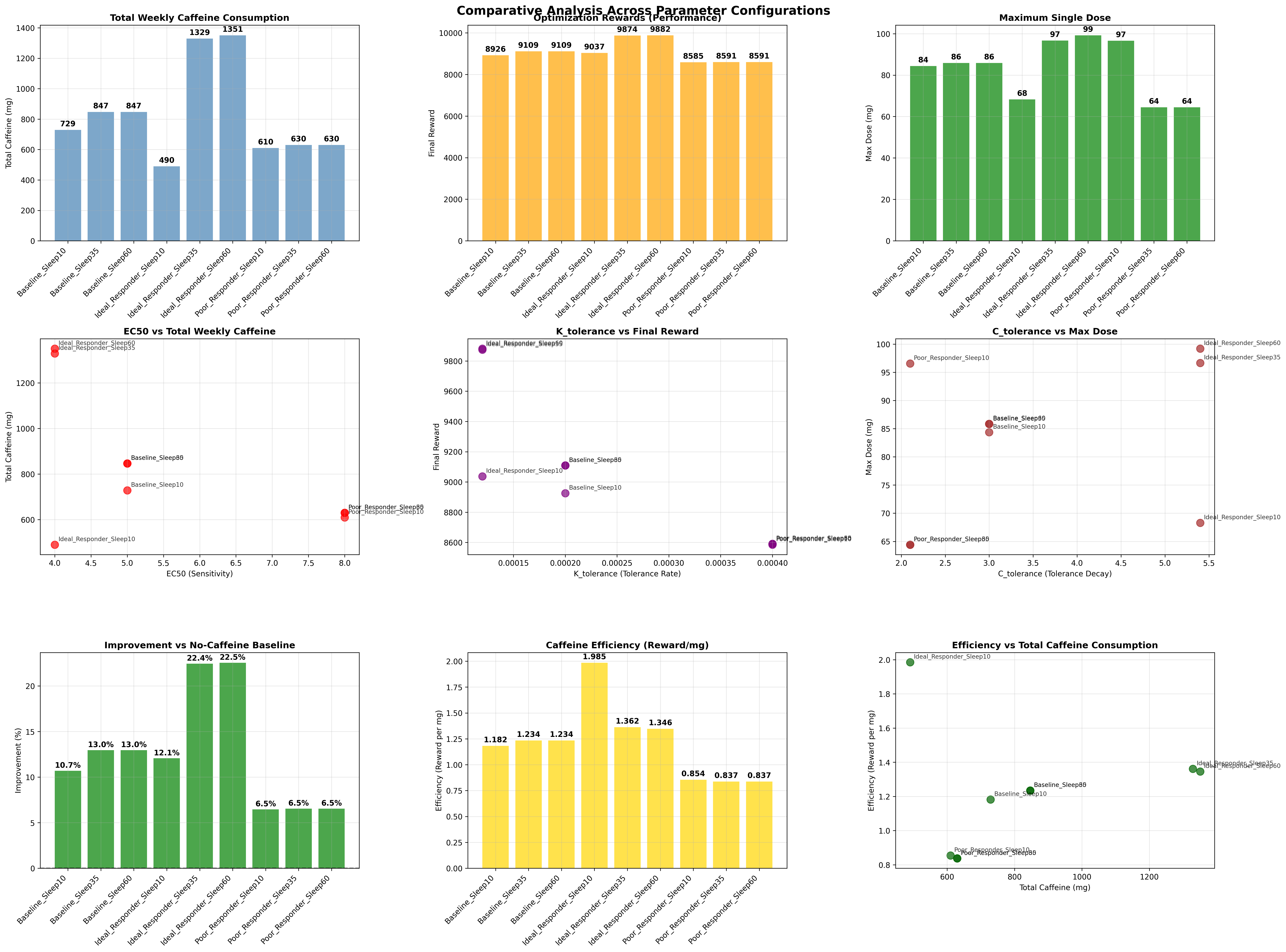
Parameter sweep

The extended study evaluates nine parameter configurations formed by crossing:

• three caffeine-response profiles,
• three sleep-disruption thresholds.

The profiles vary:

• $EC_{50}$,
• tolerance growth rate $k_t$,
• tolerance concentration parameter C_tol,
• sleep disruption threshold.

This allows the project to compare how an optimizer behaves for:

• baseline responders,
• more favorable response profiles,
• poorer response profiles,
• stricter or looser sleep sensitivity assumptions.

Result generation

The analysis code writes:

• per-configuration schedule plots,
• daily totals,
• weekly summaries,
• JSON result data,
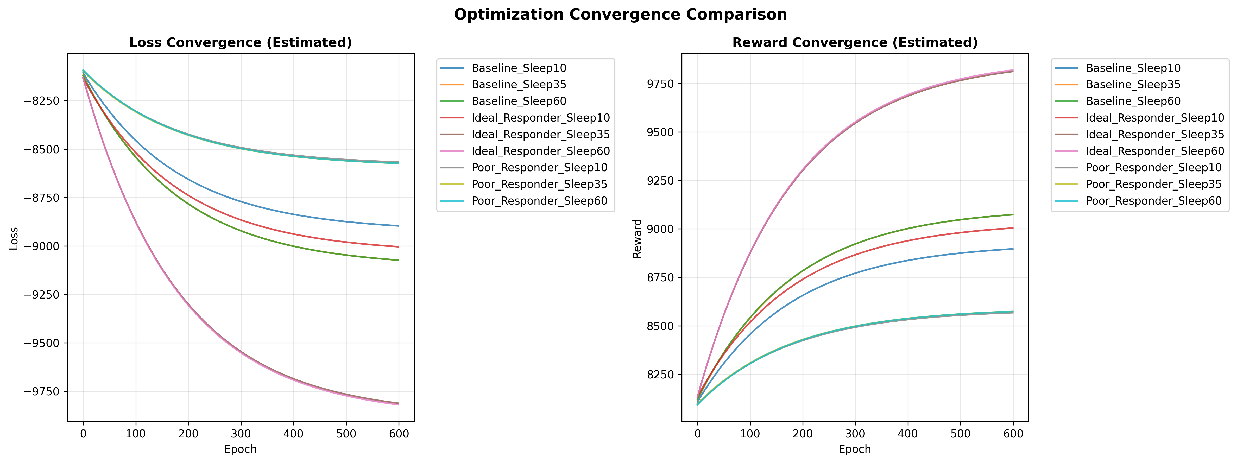
• convergence summaries,
• cross-configuration comparison charts.

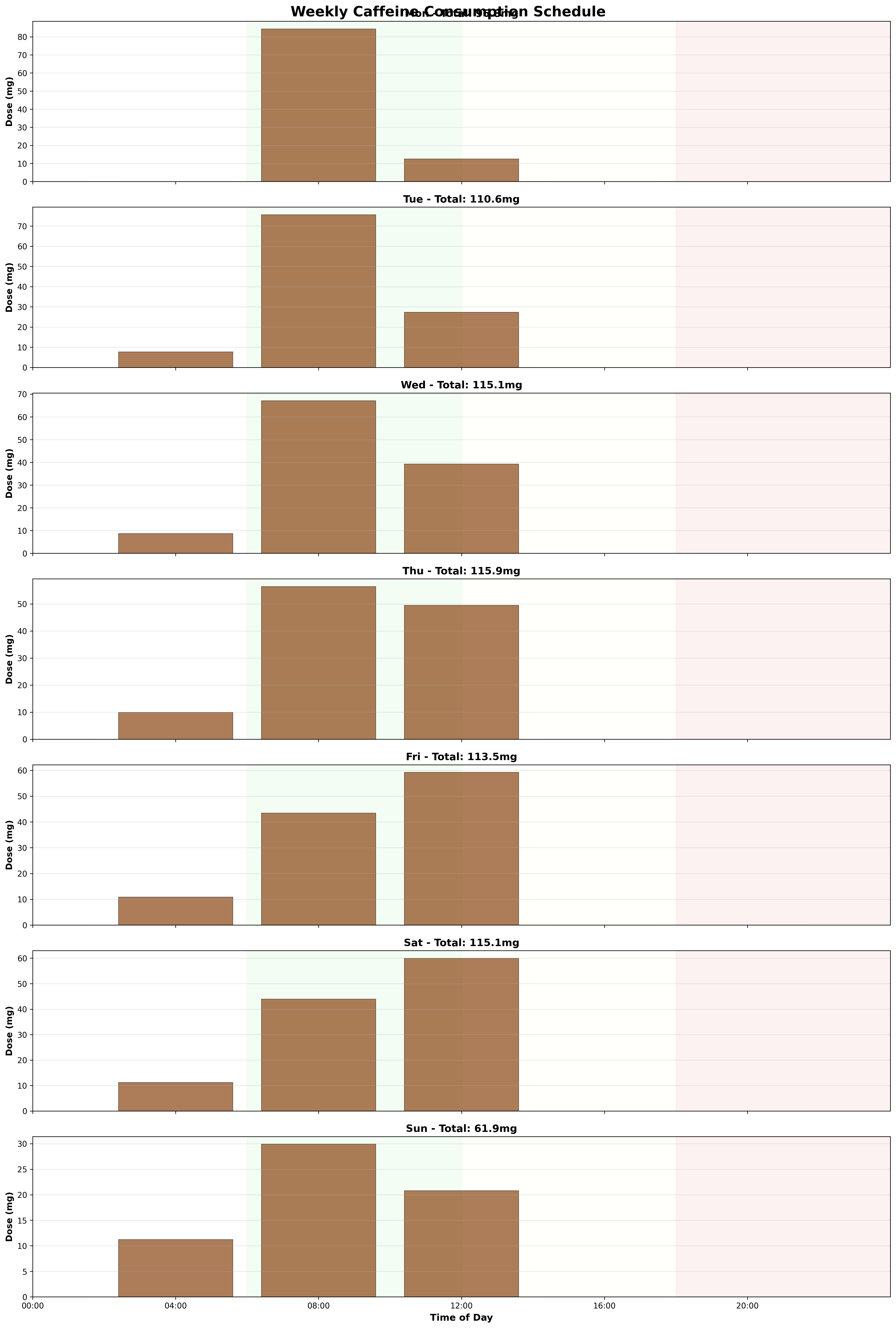
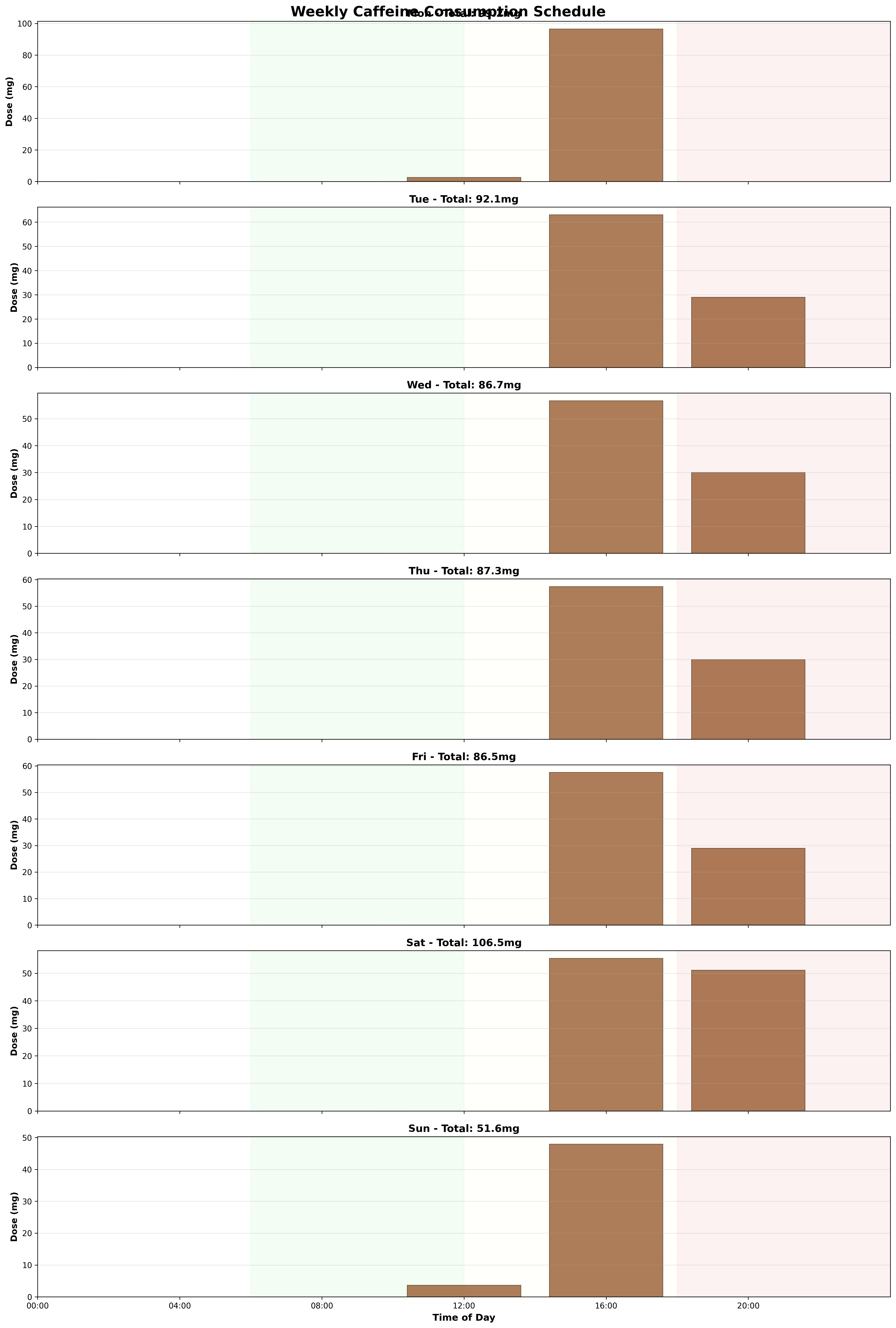
Example optimized schedules

The result folders contain separate schedules for each parameter choice. Two examples are shown below: